Audio Basics
What Does the Unit kHz Mean in Digital Music?
kHz is short for kilohertz, and is a measurement of frequency (cycles per second).
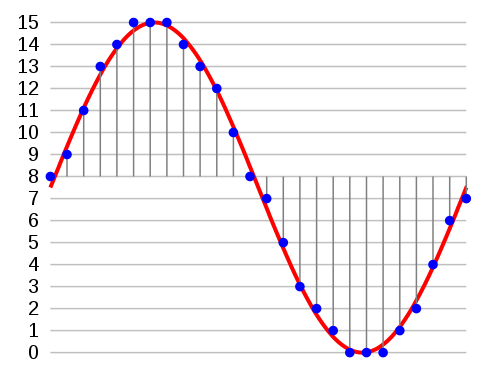
In digital audio, this measurement describes the number of data chunks used per second to represent an analog sound in digital form. These data chunks are known as the sampling rate or sampling frequency.
This definition is often confused with another popular term in digital audio,
called bitrate (measured in kbps). However, the difference between these two terms is that bitrate measures how much is sampled every second (size of the chunks) rather than the number of chunks (frequency).
Note: kHz is sometimes referred to as sampling rate, sampling interval, or cycles per second.
What is the Mel scale?
The Mel scale relates perceived frequency, or pitch, of a pure tone to its actual measured frequency. Humans are much better at discerning small changes in pitch at low frequencies than they are at high frequencies. Incorporating this scale makes our features match more closely what humans hear.
Audio Features
- We start with a speech signal, we’ll assume sampled at 16kHz.
- Frame the signal into 20-40 ms frames. 25ms is standard.
- This means the frame length for a 16kHz signal is 0.025*16000 = 400 samples.
- Frame step is usually something like 10ms (160 samples), which allows some overlap to the frames.
- The first 400 sample frame starts at sample 0, the next 400 sample frame starts at sample 160 etc. until the end of the speech file is reached.
- If the speech file does not divide into an even number of frames, pad it with zeros so that it does.
- Audio Signal File : 0 to N seconds
- Audio Frame : Interval of 20 - 40 ms —> default 25 ms —> 0.025 * 16000 = 400 samples
- Frame step : Default 10 ms —> 0.010 * 16000 —> 160 samples
- First sample: 0 to 400 samples
- Second sample: 160 to 560 samples etc.,
25ms    25ms   25ms   25ms …  Frames
400     400    400    400  …  Samples/Frame

|—————|—————|—————|—————|—————|—————|—————|————-|

|—|—|—|—|—|—|—|—|—|—|—|—|—|—|—|—|—|—|—|—|—|—|—|—|—|—|—|—|

10 10 10 10 … Frame Step
Bit-depth = 16: The amplitude of each sample in the audio is one of 2^16 (=65536) possible values. Samplig rate = 44.1 kHz: Each second in the audio consists of 44100 samples. So, if the duration of the audio file is 3.2 seconds, the audio will consist of 44100*3.2 = 141120 values.
Still dont get it? Consider the audio signal to be a time series sampled at an interval of 25ms with step size of 10ms
Check out this jupyet notebook @ https://timsainb.github.io/spectrograms-mfccs-and-inversion-in-python.html
Forked version @ https://github.com/dhiraa/python_spectrograms_and_inversion
Mel Frequency Cepstral Coefficient (MFCC) tutorial
Reading Audio Files
The audios are Pulse-code modulated with a bit depth of 16 and a sampling rate of 44.1 kHz
- Bit-depth = 16: The amplitude of each sample in the audio is one of 2^16 (=65536) possible values.
- Samplig rate = 44.1 kHz: Each second in the audio consists of 44100 samples. So, if the duration of the audio file is 3.2 seconds, the audio will consist of 44100*3.2 = 141120 values.
Audio Features
- Zero Cross Rate
- Energy
- Entropy of Energy
- Spectral Centroid
- Spectral Spread
- Spectral Entropy
- Spectral Flux
- Spectral Roll off
- MFCC
- Chroma Vector
- Chroma Deviation
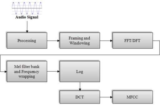
Introduction to MFCC
Before the Deep Learning era, people developed techniques to extract features from audio signals. It turns out that these techniques are still useful. One such technique is computing the MFCC (Mel Frquency Cepstral Coefficients) from the raw audio. Before we jump to MFCC, let’s talk about extracting features from the sound.
If we just want to classify some sound, we should build features that are speaker independent. Any feature that only gives information about the speaker (like the pitch of their voice) will not be helpful for classification. In other words, we should extract features that depend on the “content” of the audio rather than the nature of the speaker. Also, a good feature extraction technique should mimic the human speech perception. We don’t hear loudness on a linear scale. If we want to double the perceived loudness of a sound, we have to put 8 times as much energy into it. Instead of a linear scale, our perception system uses a log scale.
Taking these things into account, Davis and Mermelstein came up with MFCC in the 1980’s. MFCC mimics the logarithmic perception of loudness and pitch of human auditory system and tries to eliminate speaker dependent characteristics by excluding the fundamental frequency and their harmonics. The underlying mathematics is quite complicated and we will skip that. For those interested, here is the detailed explanation.
FFT/STFT Cheat Sheet:
- FFT: Fast Fourier transformA method for computing the discrete Fourier transform of a signal. Its “fastness” relies on size being a power of 2.
- STFT: Short-time Fourier transform A method for analyzing a signal whose frequency content is changing over time. The signal is broken into small, often overlapping frames, and the FFT is computed for each frame (i.e., the frequency content is assumed not to change within a frame, but subsequent analysis frames can be compared to understand how the frequency content changes over time).
- IFFT: Inverse Fast Fourier transform Takes a spectrum buffer (a complex vector) of N bins and transforms it into N audio samples.
- FFT size: The number of samples over which the FFT is computed; also the number of “bins” that comprise the analysis output.
- Bin: The content of a bin denotes the magnitude (and phase) of the frequency corresponding to the bin number. The N bins of an N-sample FFT evenly (linearly) partition the spectrum from 0Hz to the sample rate. Note that for real signals (including audio), we can discard the latter half of the bins, using only the bins from 0Hz to the Nyquist frequency.
- Window function: Before computing the FFT, the signal is multiplied by a window function. The simplest window is a rectangular window, which multiplies everything inside the frame by 1 and everything outside the frame by 0. However, in practice, we choose a smoother window function that is 1 in the middle of the window and tapers to 0 or near-0 at the edges. The choice of window depends on the application.
- Zero-padding: It is common practice to use a smaller window size than FFT size, then “zeropad” all the samples that lie in between the edges of the window and the edges of the FFT frame.
- Hop size: In STFT, you must decide how frequently to perform FFT computations on the signal. If your FFT size is 512 samples, and you have a hop size of 512 samples, you are sliding the analysis frame along the signal with no overlap, nor any space between analyses. If your hop size is 256 samples, you are using 50% overlap. The hop size can be small (high overlap) if you want to very faithfully recreate the sound using an IFFT, or very large if you’re only concerned about the spectrum’s or spectral features’ values every now and then.
Videos
- https://youtu.be/1RIA9U5oXro
- https://youtu.be/PjlIKVnKe8I